Signature File
In this example of basic classification of an area will be accomplished through the use an aerial photograph. The photograph has already been georeferenced. The photograph used must have some basic parameters to insure that objectives of the lesson are met. Through the use of this photograph basic characteristics will be classified, such as grass, asphalt pavement, concert, dirt, trees, roof tops, etc. At least 10 unique classes must be identified within the image, but more may be used. For example there may be three different types of roofs such copper, asphalt shingles, and flat office building, or multiple types of pavement. Shadows effects our ability to classify an image correctly, the less shadows the better, therefore flight paths during the middle of the day in summer are ideal to eliminate shadows.
Flying an area in summer is not idea in general because there is more vegetation which can obscure other features unless the research is specific looking for vegetation. Note the time of the year in which the flight occurred, so a determination can be made if the leaves were on or off for deciduous trees and foliage. It will also affect the colors of grass as some grasses brown in the fall and winter. The image should be with no snow cover, and basic research of the type of weather that has occurred prior to the flight is helpful in get a clear understanding of the image being used.
Flying an area in summer is not idea in general because there is more vegetation which can obscure other features unless the research is specific looking for vegetation. Note the time of the year in which the flight occurred, so a determination can be made if the leaves were on or off for deciduous trees and foliage. It will also affect the colors of grass as some grasses brown in the fall and winter. The image should be with no snow cover, and basic research of the type of weather that has occurred prior to the flight is helpful in get a clear understanding of the image being used.
Basic Parameters:
- Must be a four band image, with Red, Green, Blue, and near Infrared.
- Resolution of the photograph must be at least 1 foot but maybe smaller.
- The image must have a projection.
- The image used should be of a section of a city or rural area but not multiple miles in size.
It is suggested that for learning the processes that the same image be used as that used by the author for this lesson. The image used is located on an image server and is an image of Louisville, Jeffererson County, Kentucky and was flown in the spring of 2012. Note these aircraft files are very large when broken into tiles. You must use the service to have the four bands required in this exercise or locate another image file containing four bands. The individual images can be downloaded in a zipped format without the IR band, which will not work for this exercise. The individual images can be downloaded and viewed without the requirement for a mapping software program, at: ftp://ftp.kymartian.ky.gov/kyaped/lojic2012/.
Process:
The first part of the process will be preparing the image for the analysis. To start the project open ArcMap and place a shapefile or basemap of Louisville, KY; zoom into the downtown area.
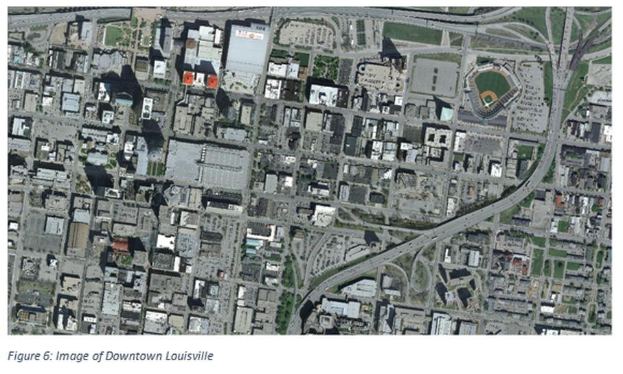
Load the image service into ArcMap which is located at: http://kyraster.ky.gov/arcgis/rest/services; remember this is not a URL for a web browser but must be connected to as an ArcGIS Server via ArcCatalog or Add Data. Once connected you will need to go to the ImageService folder and then find KY LOJIC 2012 6IN. Note there are many other image services on this server. Once the Image has been loaded the basemap information may be removed, as this was done just to zoom you into an area. Zoom to a region of the downtown approximately like the image in Figure 6. The scale is 1:3,000, it can be even smaller than this since only a few city blocks are required. Do a visual inspection of the image to better understand the type of information that is available for the analysis that will be created. Visual identify items in the image such as trees, green areas, streets, parking lots, different types of roof tops, etc. Also identify the shadows in the image as this will affect the classification of items. The top of the image is north and thus the sun is always to the south creating shadows that are from the bottom of the image to the top. Also you will see some shadows that going from the right side to the left, which meant the image must have been taken prior to solar noon. The area represented in the image is of downtown Louisville, KY I-65 is the major north-south highway and I-64 is near the north edge of the image. The baseball stadium is home to the Louisville Bats. The Ohio River is just nort of I-64 The curves on I-65 ae known as hospital curve. In general Louisville has a grid of north and south and east-west streets.
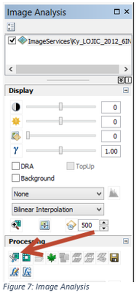
The next part of this process will be the capturing of the image shown in Figure 6, make sure the zoom is at the level needed for the analysis. Go to the Window tab and select Image Analysis and a toolbox should appear. Highlight the name of the Image Service, then click on the button which the red arrow is point toward in Figure 7. This will perform a clip of the image out of the service visible on the screen. This will complete the clip, the file has not been saved and if not saved it is only a temporary file and will be lost for future use. Click on the Disk Icon on the far right side and save thei mage. The image may take few minutes to save depending on the computer and the process running on the computer. At this point you can turn off the service or remove it which will allow your image to refresh at a quicker rate and will not be dependent on the internet. Close the Image Analysis Window.
Open the property window for your clip and select the Symbology Tab. The Symbology information appears very different from the typical window for a shapefile.
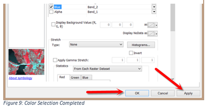
One of the first task to complete is switching the displayed colors, ArcGIS Desktop only allows three colors to be displayed at one time, thus the default is to display Red, Green and Blue and thus making no usage of the near infrared band, which is band 4. For this work a re-arrange of the spectral bands will be done. Band 1 (red) will become Band 4 (IR), Band 2 (green) will become Band 1 (red), Band 3 (blue) will become band 2 (green).
Open the property window for your clip and select the Symbology Tab. The Symbology information appears very different from the typical window for a shapefile.
One of the first task to complete is switching the displayed colors, ArcGIS Desktop only allows three colors to be displayed at one time, thus the default is to display Red, Green and Blue and thus making no usage of the near infrared band, which is band 4. For this work a re-arrange of the spectral bands will be done. Band 1 (red) will become Band 4 (IR), Band 2 (green) will become Band 1 (red), Band 3 (blue) will become band 2 (green).
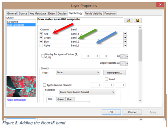
Once these changes have been made click Apply and then OK. It will take a few moments to regenerate the image with the false colors red for IR that you have selected. The larger your initial image the longer it takes regenerate the image and computer speed also effects the process.
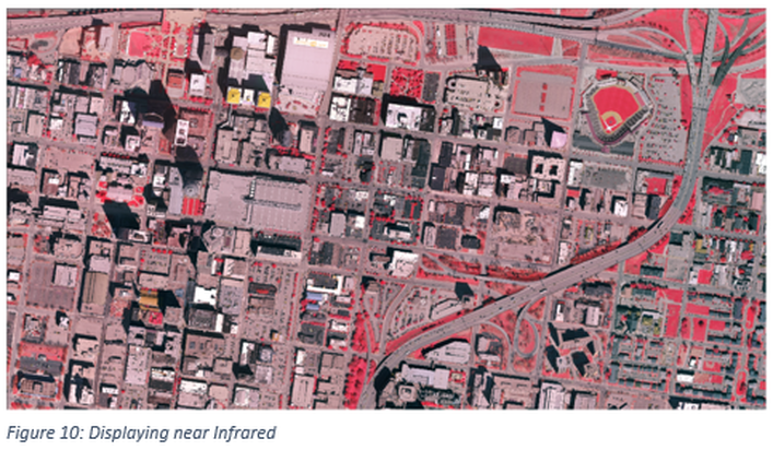
Areas that was vegetation now appears to be red in color in general, this is the result of the near IR band, and vegetation having lots of reflectance in the near IR region of the electromagnetic spectrum. Something that is blue in color disappears from this image since band 3 is not being used, this true for something having blue wavelength as a major component. This is not a statistical analysis but gives a feel for different types of surfaces. The areas that are red are emitting large amounts of near infrared and this is an indication of vegetation. The near IR band is specifically useful for determining vegetation. Do not confuse this band with that of thermal IR.
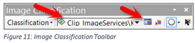
The next component will be to develop a spectral signature for different types of surfaces and then complete an analysis of the surface. This spectral signature could be done with all four bands. Add the Image classification toolbar to your map. You can dock the toolbar or leave it floating. This tool will require the use of visual inspect and use the classification tool to classify large areas of your image. The signature file can be saved and used with other parts of this image that are outside of the clipped area and potentially other images.
The next component will be to develop a spectral signature for different types of surfaces and then complete an analysis of the surface. This spectral signature could be done with all four bands. Add the Image classification toolbar to your map. You can dock the toolbar or leave it floating. This tool will require the use of visual inspect and use the classification tool to classify large areas of your image. The signature file can be saved and used with other parts of this image that are outside of the clipped area and potentially other images.
Use the pull down to make sure your image file (the clipped one) is the one showing in the window. Then click on the first button to the right of the file location to open the Training Sample Manager, see Figure 11. The word training refers to the fact that the software is learning the different classification from the image. The next to last button has a pull down, which gives a choice of how the sample will be selected, circle, rectangle or polygon, currently circle is selected, but any one of the three can be used, the author will use the polygon in this example. The selected sample the area should be relatively small.
The Training Sample Manager shown in Figure 11, will be blank, zoom to the area of the image to make the first selection. Zoom to a field that appears to be covered with grass (remember this image was taken in spring and the grass has not fully turned green. Draw a polygon and finish the polygon by a double click. When completed the first line in the training manager should now have content. Create additional polygons of similar features insure that you know what each feature represents, since generic names will be initially generated. It is possible to merge features together, name the features appropriately and change the display color.
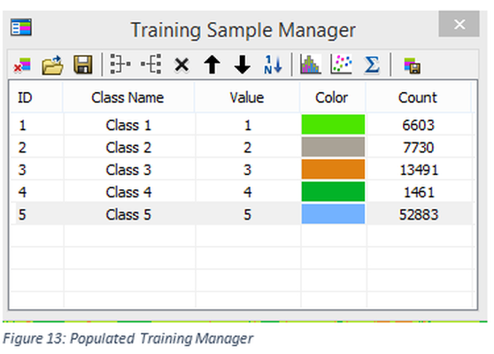
In figure 13, is a representative classification of different areas on the map, for an actual classification of this particular image more than five classes would be made for maximum accuracy. The count number on the right side is the number of pixels represented in each training sample. Since the resolution of the image is 6 inches, each pixel represents a 6 inch by 6 inch square or ¼ square foot. This is a very small area compared to the total area of the image. The colors represented in Figure 13 will be the initial classification of colors on the classification is done, the colors can be changed in the symbology tab of the Properties window.
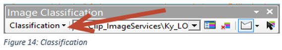
Once the samples have be finalized the next component must be done using the toolbar which is the construction of the classification. Using the pull down arrow under classification to select a methodology, as seen in Figure 14. The method used for this type of classification is the Interactive Supervised and it may take a short period of time to see the results, depending on computer speed and memory. A new shapefile will be created. If after the classification is displayed areas are inaccurately classified, then additional training sample can be made and others deleted to improve the classification. It may also mean for example that there are multiple roof classifications or vegetation to refine the processes. For example trees need to be classified different than turf. If water features are included in the image that also causes potential issues if the IR band is used in the classification. After making modifications to the sample file, the classification will need to be run again which will create another shapefile. Once the classification is acceptable remove all the shapefiles that were created during the classification process, keeping only the final example. Besides the Interactive Supervised classification methodology there are other classification which can be selected. Some of these methods require the use of the signature file which was created. Therefore, the already created signature file can be saved in the training manager window. This image does have problems with shadows.
All classification methods will provide the number of pixels for each classification (except Interactive Supervised) thus the area of each type of classification can be determined. Since each pixel is 6 inches by 6 inches or a quarter of a square foot. Since most of the classifications create a shapefile the user can also change the symbology as needed, colors should be selected that are descriptive.
There are other types of classification NDVI which is specifically designed for the classification of vegetation and can only used with four band data. Realize that not all images have the fourth band of near IR. For those devices without the forth band, classifications can still be done (not NDVI) utilizing the same methods as previous discussed. In the remote sensing class classification methodologies will be covered in more depth. Experiment with the different classification methods under the Classification pull down.

