Buffering Dissolved
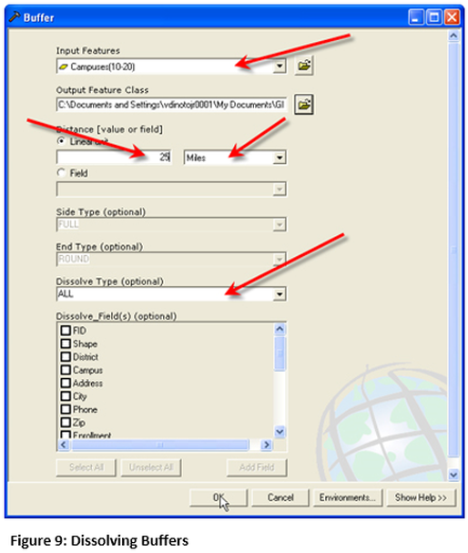
In the first part buffers were arranged on top of other buffers. A better way to present the same data set would be to dissolve the rings so they do not overlap. To accomplish this task a new buffer will be created around the KCTCS campus point shapefile. Open the buffering tool in the Toolbox again. The inputs for the first, third and fourth dialog boxes will be the same as in the initial buffering process. For the second dialog box a new shapefile should be created so a new descriptive name must be inputted with an appropriate storage location. The buffer window has been expanded to see all of the different parameter that can be controlled. Near the bottom of the window is the Dissolve Type. The default is "None", which means that no dissolve created as could be seen in the first example. The dissolve type will change to “All”.
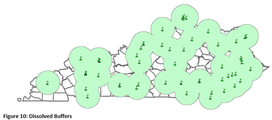
The result of having buffering with dissolve selected is that the circles no longer overlap, but where they touched have been blended together. The country boundary shapefile needs to be placed above the buffer layer and made hollow. Note the information extends outside of the state boundary because the data has not been clipped for this layer. The next step would be to clip the data, as shown previously for better map construction. The same type of process can be done for lines or polygons. It is very important for good data management that unneeded shapefiles be deleted from both the map and the storage location, because each time a buffering process is done, a new shapefile is created.
Clipping
Since KCTCS institutions are in Kentucky only (students do come from neighboring states but service areas are within Kentucky). The buffers should remain within the state boundaries there for the feature will need to be clipped. For additional information about clipping see the technical skills lesson on this topic. The clip tool is located in the Toolbox under the Analysis Tools in the Extract Tray.
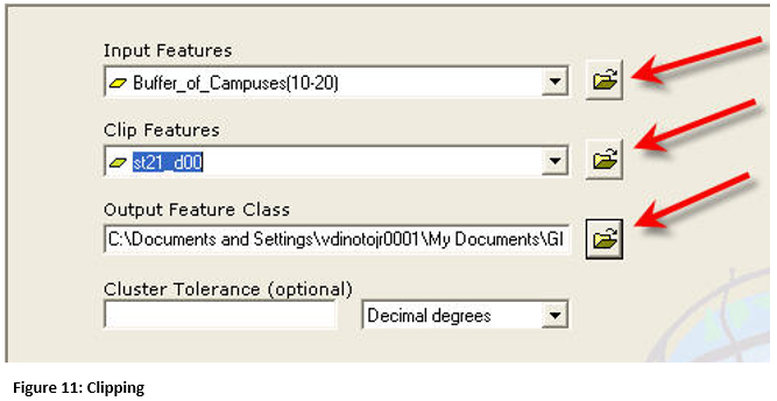
The clip window requires a file to be clipped and a polygon boundary to clip against. Our file will be the recently created buffer file and the boundary will be the state boundary file. Since both of these files are loaded the pull down arrow was used for the selections. The third window is the location in which the new shapefile will be stored. The storage location and the naming convention should covey the appropriate information. The remaining items in the clip window will use the default values.
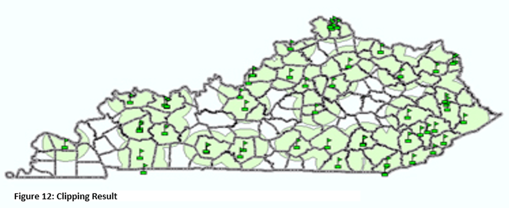
The results of clipping against the state boundary can be seen in Figure 12: Clipping Result. Figure 9: Dissolving Buffers The county boundary file has been made hollow and placed above the buffer layer. The result of this clipping operation is the creation of a new shapefile, therefore the original buffer shapefile can be removed. Editor’s note: a couple college campuses in southern Kentucky appear to be in Tennessee, this because the center of the symbol is located at the campus point.

