ArcMap Desktop
Load the Kentucky County file or another basemap layer as discussed previously. Have only the county basemap turned on to simplify the view as the geocoding process is begun. The Excel data file can be loaded into ArcMap or the location of the Excel file selected.
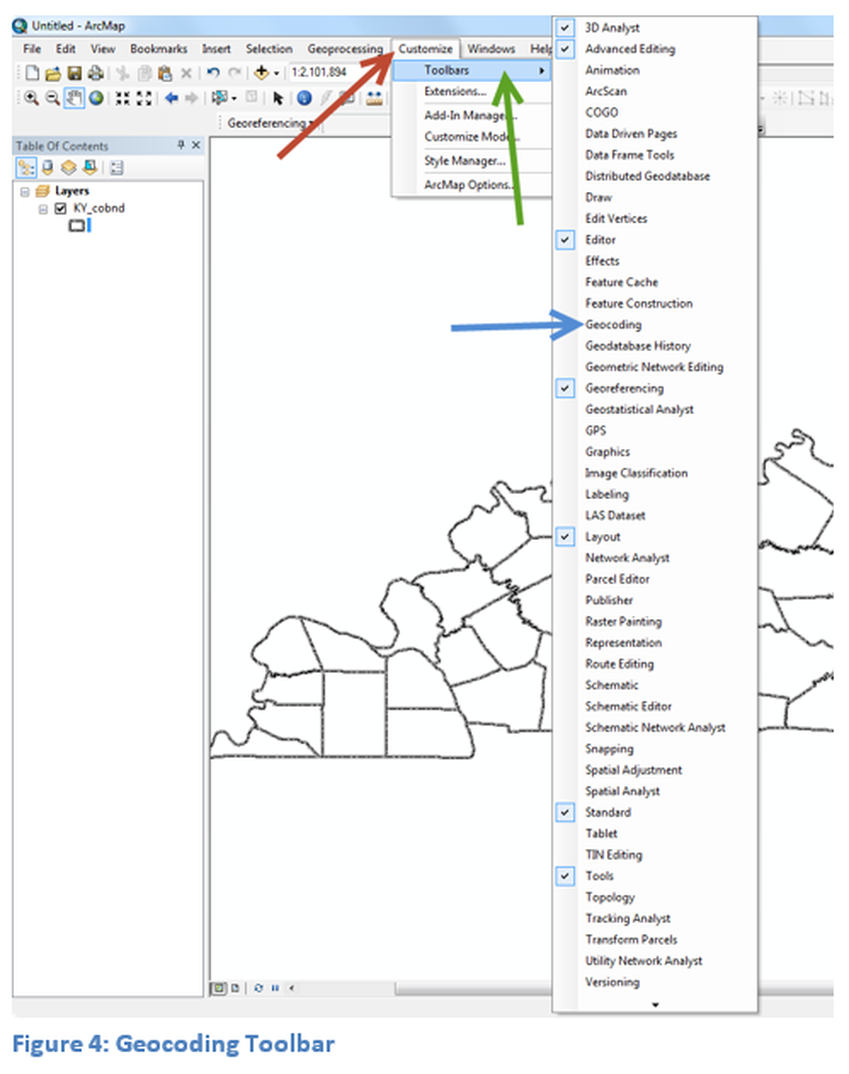
Click on Customize and select Toolbars, in toolbar menu select Geocoding. Once selected the Geocoding toolbar will appear. As seen in figure 4.
Click on Customize and select Toolbars, in toolbar menu select Geocoding. Once selected the Geocoding toolbar will appear. As seen in figure 4.
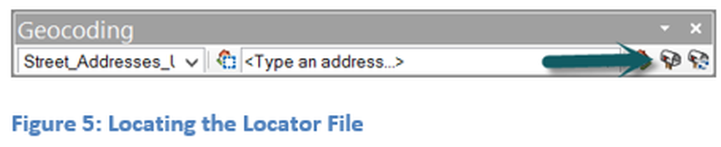
First a locator file must be selected this is done by clicking on the mailbox icon as seen in Figure 5.
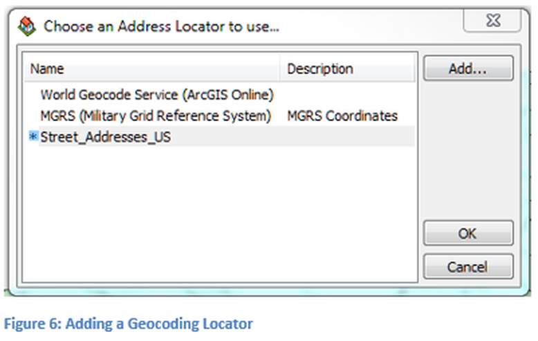
Click on the Add button to input the address of the locating service that will be utilized. See Figure 6.
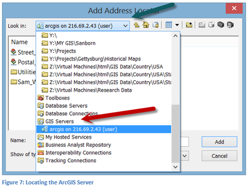
Use the pull down to select GIS Server, locate 216.69.2.43 in the list of services just select the machine and a locator will then be selected as seen in figure 8. If the machine is not visible it must be added. This is accomplished just as was in the ArcCatalog exercise. Using the following string 216.69.2.43/arcgis/services. Once the connection has been established two geocoding services should be visible as in figure 8.
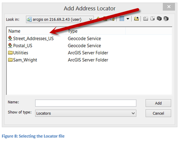
The first locator file in figure 8 is the one that should be selected for this operation. Now that the locator file has been established the geocoding process can be started.
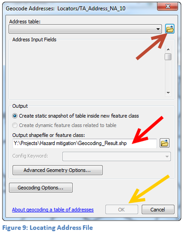
The first step is to locate the Microsoft Excel file that contains the address list that will be geocoded. Click on the file folder at the top of the window in figure 9, to locate the address file. Since Excel files contain multiple sheets, the sheet which contains the data to be geocoded must next be selected. The address field data should appear in the window shown in figure 10. The address data file will not be modified with the location data instead a new shapefile will be created in the geocoding process. The output shapefile location and name must be defined. The default location and name appears near the red arrow. Select OK to continue the process.
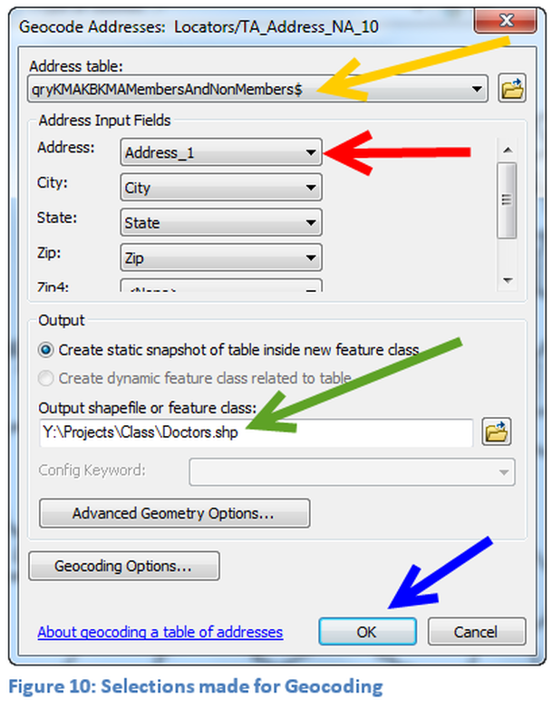
The Address table, shows the name of the file to be geocoded, which is the name of the doctor’s worksheet. In the Address field the pull down was used to locate the Address_1 field, since the program did not recognize the location for the street addresses. The other fields were automatically identified since the names used in the Excel spreadsheet were the same as those the geocoding program used. The purpose of this step is to insure that the proper fields in the locator and the address file are compared. Naming fields with the default names will speed up the process. The green arrow is pointing to the name and storage location of the output shapefile. Using just the default name does not help to identify what is contained within the shapefile and is not good file management. Once all the fields have been completed begin the geocoding process. Remember an internet connection is required to connect to the locator file and the greater the bandwidth of the connection the faster the process will be done.
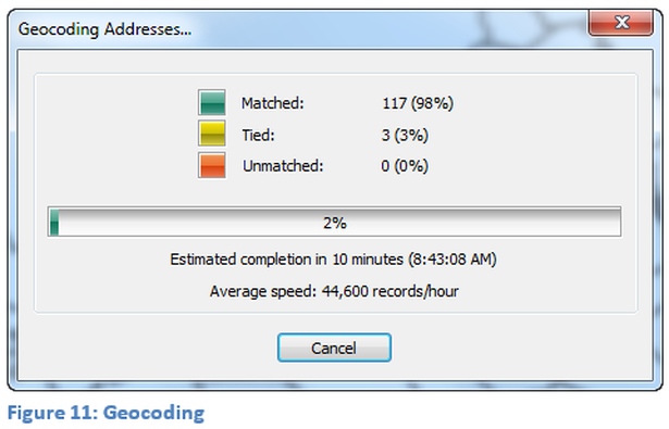
Figure 11 shows the progress window of the geocoding process. The software uses a predefined threshold as a starting point which can be modified and re-coded for greater or lesser accuracy. The ‘tied’ designation is for those data points at the threshold level.
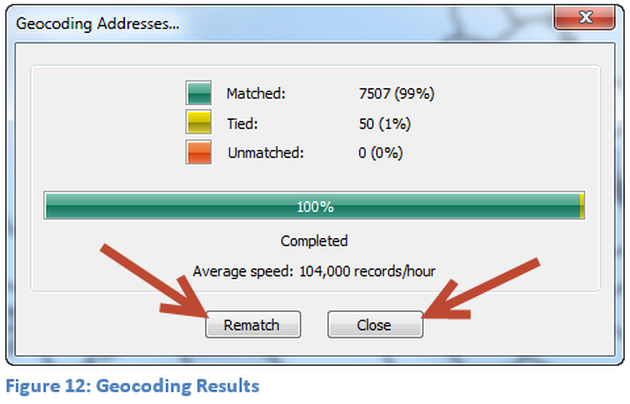
Figure 12 shows the final results of the geocoding process. Note for this particular data set of more than 7500 addresses they were either matched or tied and no data was unmatched. The newer locator files do a better job of matching data. Two options are available, rematch or close. When close is selected the data will appear on the map
For this example a rematch will not be necessary, because there was no unmatched data. But it is important to understand what can be done in the rematch window. If rematch is selected the rematch window in Figure 13 will appear.
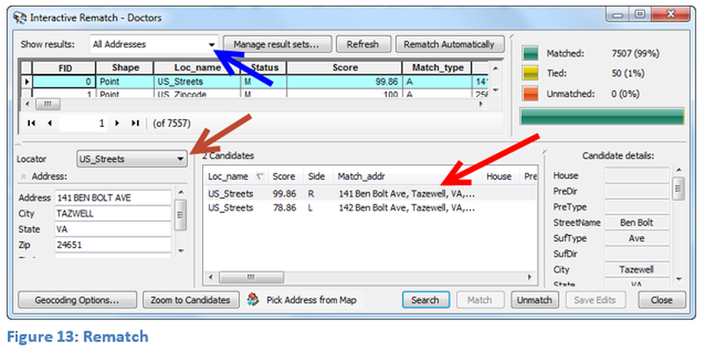
There are several factors which can be controlled, which include an automatic rematch or a manual rematch. The brownish colored arrow points to the locator file. Geocoding against a different locator, for all the data or just a part of the data set, like the unmatched data can be done. The blue arrow points to the data set or the part of the data that action would occur, currently all addresses are being displayed. Only the unmatched addresses can be selected by using the down arrow. Manually selecting the match is being pointed to by the red arrow. There are additional options that can be controlled such as changing the threshold for the matching. If the purpose of the map is to look at city level data a fairly high threshold is required, for a larger scale map such as a multi-state region then a lower threshold can be used for the match.
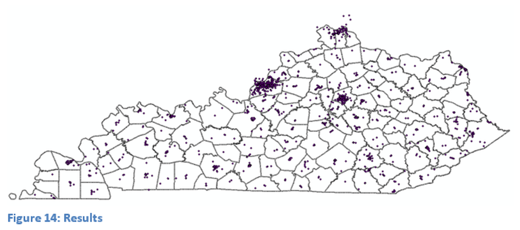
As can be seen in the Kentucky map in figure 14, there are areas of concentrations of doctors and areas with very few doctors. This map is a little misleading because many physicians’ offices contain multiple doctors and on the map they show up as a single point since they are plotted on top of each other, i.e. two or more points with the same latitude and longitude will show as only a single point. It is not an error that some of the data points are outside of the state of Kentucky. The Kentucky Medical Association has memberships outside of Kentucky.

